Project estimations with Monte Carlo Analysis
The estimation process in project management is quite an important activity because many decisions depend on its precise completion. It is quite challenging considering all the different factors impacting the project’s execution. That is why there are various techniques which can help us create our estimations.
In this article we will have a brief look at the most common practices according to PMI and we will pay special attention to those of them based on mathematical approach.
Estimation Techniques
- Analogous estimating – we compare our current project with past similar ones. This technique is also known as “top-down”. We should be careful with it because sometimes it’s not very accurate. analogous2

-
Parametric estimating – we estimate the unit cost/duration per activity and then the number of units required for completing it, e.g. $10/hour or 3 days/module. The measurement, however must be scalable, otherwise we risk to lose accuracy.
-
Bottom-up estimating – we have concrete information about the atomic activities, so we can estimate them in lowest level, then easily combine them in order to get estimation for the composed activities and thus for the entire project. This approach might be very time consuming, so it needs special attention when it comes to lager projects.
-
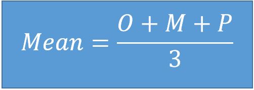
Three-point estimation – this technique considers the risk and uncertainty by taking in mind estimations for the optimistic, pessimistic and most-likely outcomes:

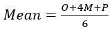
We can use it by identifying values for optimistic (best-case scenario), pessimistic (worst-case) and most-likely values of the current task. After that we can calculate the formula for receiving more accurate result for the Mean - the technical definition of “average” value.
- Three-point estimation – PERT – variation of 3-point estimation where we have again the values for Optimistic, Pessimistic and Most-likely estimation. The difference lies in the formula where we calculate the most-likely value with different weight.
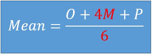
Based on the Beta distribution, this statistically proven formula will give us more realistic result of the Mean.
We can also calculate the standard deviation – “σ”, which measures the amount of variation from the mean. This can be quite useful when we measure the risk of the uncertainty, but this is a topic for another article :)

The last two techniques are really common in the project management world, but unfortunately they give us only rough estimations. There are times when we need a justification of the decision we have made and this simple formula would not be enough.
This is where the Monte Carlo Analysis comes in.
Monte Carlo Simulation
Technique, used in project management where we can calculate random project estimations within a given range, as many times as we want. This simulation is based on probability distribution and produces many different outcome values.
Now, let’s see how this estimation works…
Example
We were given the following data for completing a simple task in days. You can think of something like creating a super simple mobile application upgrade.
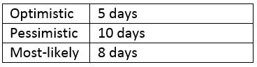
We will calculate the Mean with the techniques above and will monitor the differences
Three-Point Estimation
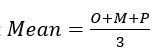 Using this formula the result for our Mean is = 7.667
PERT Estimation
Using this formula the result for our Mean is = 7.833
 Did you notice the difference between the two values? Now let’s take a look at another technique for estimation…
Monte Carlo Simulation
First we will try simple simulation of random values from 5 to 10 and apply it 500 times.
The result here for the Mean is 7.547.
You can notice that in this scenario we don’t use the most-likely value, that’s why the mean is a bit lower. However if you try it with very large numbers the difference won’t be that significant.
Note: For those of you who are interested in testing this in Excel, the formula for random number between a range is RAND()(P-O)+O this is necessary because the rand function returns a random number between 0 and 1 and this way we can use it for whatever range we want.*
Monte Carlo Simulation v2
In the next test we will use the Monte Carlo Analysis with the Triangular distribution – it will use optimistic, pessimistic and most-likely values:
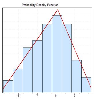
From this graphic we can notice that the values which are occurring most frequently are between 7.5 and 8.5.
The average of all the 500 random values is 7.733 a lot closer to our most-likely value. Therefore our Mean is 7.733.
Conclusion
As we tried different estimation techniques we found out that the result are approximately the same with slight difference, see below.
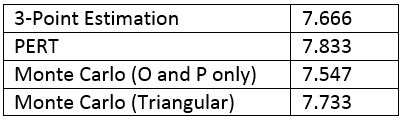
However every project is unique and it is our responsibility to find the right method and use it, but remember these estimations will never give us 100% probability.
If you like this, follow me on twitter!